Thinking about Variation
You may have heard the terms variance and standard deviation before, but you may not have thought about how they are used to describe data. In this module, we are going to discuss 1) variation, 2) the relationship between variance and standard deviation, and 3) how to interpret these properties when analyzing experimental data.
Variation
Let’s consider the data shown in Fig. 1. Here we see cholesterol levels measured on the same sample using two different techniques: an autoanalyzer[1] and the microenzymatic[2] method.
The average cholesterol level for each data set is 200 mg/dL (as illustrated by the dotted line). But we can see that the autoanalyzer measurements are more variable than the microenzymatic measurements. This example tells us that means (averages) alone do not contain enough information to summarize and compare data sets. We need another statistic to measure variation.
One place to start when considering variation is to find the range, which is the difference between the largest and smallest measurements in a sample (i.e. maximum value – minimum value). The range tells us the “width” of our data set.
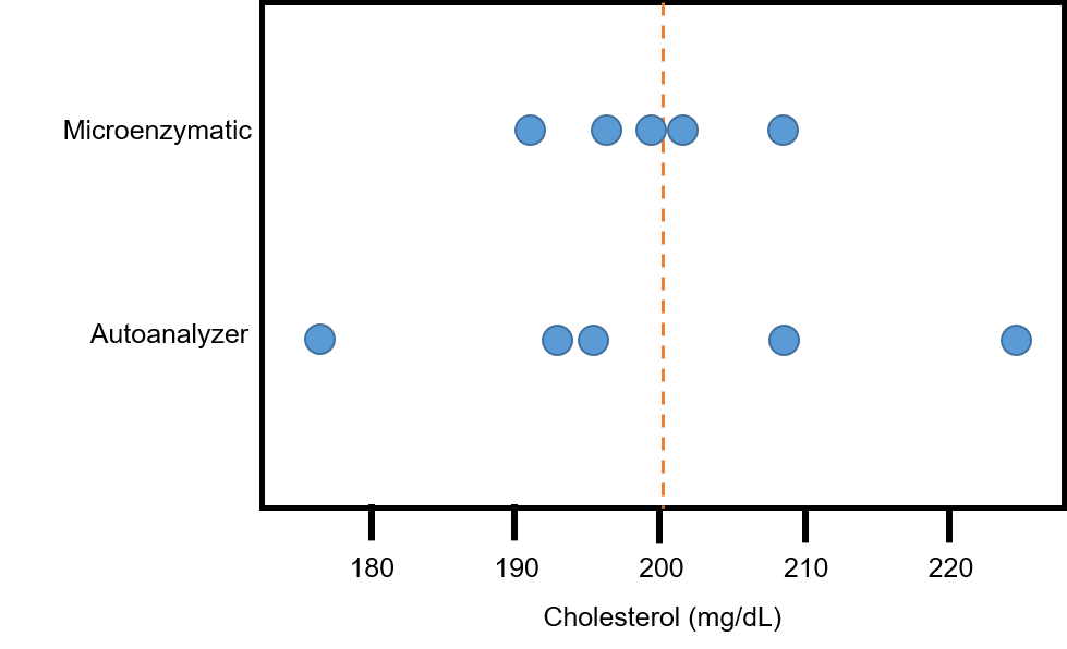
The range is straightforward to calculate, and it helps us see the spread of numbers in a data set. We need to keep in mind, though, that range is very sensitive to extreme values. Let’s do an example calculation where we find the ranges of the two sets of cholesterol measurements shown in Figure 1. We are going to find the difference between the highest cholesterol measurement and the lowest measurement for each technique.
Autoanalyzer Measurements:
The range of these data is the highest measurement (226 mg/dL) minus the lowest measurement (177 mg/dL), which equals 49 mg/dL.
Microenzymatic Measurements:
The range of these data is the highest measurement (209 mg/dL) minus the lowest measurement (192 mg/dL), which equals 17 mg/dL.
Our calculations indicate that the autoanalyzer measurements were more variable than the microenzymatic measurements. In other words, the measurements obtained by the autoanalyzer were more spread out, resulting in a wider data set, than those using the microenzymatic method.
Variance and Standard Deviation
Often, the range does not do a good job of measuring variability. Consider Fig. 2, which shows quiz scores (0-10 points) from four class sections of an introductory biology course.
In all four classes, the range is 4 and the mean is 7. However, we can see from the graphs in Fig. 2 that the four classes performed differently on this quiz. Most of the students in section 1 scored a 7; the students’ scores from section 2 were spread evenly between 5 and 9; about half the students in section 3 did very well and the other half did not do well; and in section 4, the scores were quite varied with no obvious pattern.
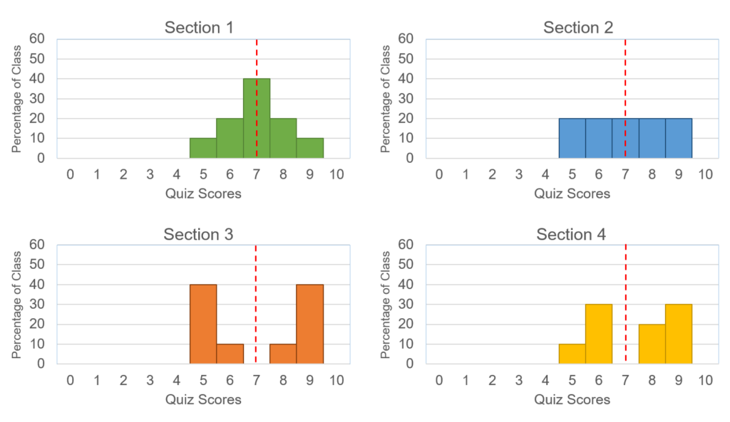
In section 1, the mean does a good job of representing the results, since most of the students scored a 7. In section 2, all scores within the range are represented equally, and the average score does not reflect the majority of scores. In sections 3 and 4, no one actually earned the average score. There were two distinct groups of scores in section 3 (high and low), but in section 4, the scores were variable above and below the mean.
To better understand and describe the data, we need a statistic that will measure the spread of our data (like range does) but that will also capture the variation within our data set, and thereby telling us how well the mean represents our data. This brings us to the topic of variance and standard deviation. These terms are very closely related. In order to calculate standard deviation, we first need to find variance. Let’s start with some definitions of these terms:
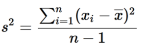
Variance is the average squared distance between each data point in our sample and the mean of our sample. It is given in squared units (s2 ). In other words, we find variance by first determining how far away from the mean each of our data points lie. We then square each of those values and take the average of all of those squared values. The formula is shown in Fig. 3, and we will go through two examples step-by-step.
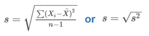
Standard deviation is the square root of the variance. Its units are given as basic units of measurement (i.e. not squared). Standard deviation represents the “typical” (though not “average”) distance between the mean and the data points in the sample. It can be thought of as measuring the spread of data. Two variations of the formula are shown in Fig. 4, and we will go through two examples.
Example Problems using Variance and Standard Deviation
Example Variance (s2 ) Calculation: Quiz Scores
Let’s take a look at the spread of data from the Section 2 class shown in Fig. 2. Suppose there were 20 students in Section 2. Based on the data in the graph, we know that the 20 individual quiz scores were:
5, 5, 5, 5, 6, 6, 6, 6, 7, 7, 7, 7, 8, 8, 8, 8, 9, 9, 9, 9
To calculate variance, we follow these steps:
STEP 1: Calculate the average for these data:
(5+5+5+5+6+6+6+6+7+7+7+7+8+8+8+8+9+9+9+9)/20 = 140/20 = 7
STEP 2: For each data point, calculate its distance from the mean, then square the result:
5-7 = -2; -2(2) = 4
5-7 = -2; -2(2) = 4
5-7 = -2; -2(2) = 4
5-7 = -2; -2(2) = 4
6-7 = -1; -1(2) = 1
6-7 = -1; -1(2) = 1
6-7 = -1; -1(2) = 1
6-7 = -1; -1(2) = 1
7-7 = 0; 0(2) = 0
7-7 = 0; 0(2) = 0
7-7 = 0; 0(2) = 0
7-7 = 0; 0(2) = 0
8-7 = 1; 1(2) = 1
8-7 = 1; 1(2) = 1
8-7 = 1; 1(2) = 1
8-7 = 1; 1(2) = 1
9-7 = 2; 2(2) = 4
9-7 = 2; 2(2) = 4
9-7 = 2; 2(2) = 4
9-7 = 2; 2(2) = 4
STEP 3: Now add up all of the results from step 2:
4+4+4+4+1+1+1+1+0+0+0+0+1+1+1+1+4+4+4+4 = 40
STEP 4: Finally, divide the result from step 3 by the total number of original data points (for a complete population), or the number of data points minus 1 (for a sample data set from a population). In this case, we will divide by 19, since we are counting scores from only a sample of all students who take introductory biology.
s2=40/19 = 2.1
Example Standard Deviation Calculation: Quiz Scores
Once we find the variance (s2), calculating standard deviation (s) requires only one more step – finding the square root of the variance!
s = √s2
s = √2.1
s = 1.45
Using these steps, we can calculate the standard deviations (SD) for the remaining class sections:
Section 1, SD=1.12
Section 2, SD=1.45
Section 3, SD=1.89
Section 4, SD=1.52.
What do these values tell us? The smaller the standard deviation, the better the mean represents the data.
Why do we need standard deviation if we know the variance? The units of standard deviation are “regular” (not squared) units and a bit nicer to handle.
Example Variance (s2 ) Calculation: Tetrahymena Food Vacuoles
Let’s consider a data set that includes the number of food vacuoles formed in 12 individual Tetrahymena cells after adding black ink to the cell culture medium. The number of food vacuoles we count in the 20 cells are: 5, 8, 5, 9, 10, 4, 7, 6, 9, 7, 6, 8, 6, 7, 7, 8, 6, 3, 11, 8.
To calculate variance, we follow these steps:
STEP 1: Calculate the average for these data:
(5+8+5+9+10+4+7+6+9+7+6+8+6+7+7+8+6+3+11+8)/20 = 140/20 = 7
STEP 2: For each data point, calculate its distance from the mean, then square the result:
5-7 = -2; -2(2) = 4
8-7 = 1; 1(2) = 1
5-7 = -2; -2(2) = 4
9-7 = 2; 2(2) = 4
10-7 = 3; 3(2) = 9
4-7 = -3; -3(2) = 9
7-7 = 0; 0(2) = 0
6-7 = -1; -1(2) = 1
9-7 = 2; 2(2) = 4
7-7 = 0; 0(2) = 0
6-7 = -1; -1(2) = 1
8-7 = 1; 1(2) = 1
6-7 = -1; -1(2) = 1
7-7 = 0; 0(2) = 0
7-7 = 0; 0(2) = 0
8-7 = 1; 1(2) = 1
6-7 = -1; -1(2) = 1
3-7 = -4; -4(2) = 16
11-7 = -3; -3(2) = 9
8-7 = 1; 1(2) = 1
STEP 3: Now add up all of the results from step 2:
4+1+4+4+9+9+0+1+4+0+1+1+1+0+0+1+1+16+9+1 = 67
STEP 4: Finally, divide the result from step 3 by the total number of original data points (for a complete population), or the number of data points minus 1 (for a sample data set from a population). In this case, we will divide by 19, since we are counting food vacuoles from just 20 cells, which is a small subset of the total population of cells in the world.
s2=67/19 = 3.5
Example Standard Deviation Calculation: Tetrahymena Food Vacuoles
Once we find the variance (s2), calculating standard deviation (s) requires only one more step – finding the square root of the variance!
s = √s2
s = √3.5
s = 1.87
What does the standard deviation tell us in the case of Tetrahymena food vacuoles? In this case, the standard deviation tells us how spread out our data are, that is, how well the mean food vacuole count represents the number of food vacuoles we would find if we were to count them in many more Tetrahymena cells. The larger the standard deviation, the larger range in the number of food vacuoles we would expect to find in additional Tetrahymena cells.
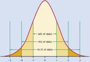
If we plot the number of food vacuoles that we count amongst many Tetrahymena cells, and our data tend to cluster around the mean and fall away from the mean about equally on both sides, we can also apply something called the Empirical Rule, which is described below.
The Empirical Rule
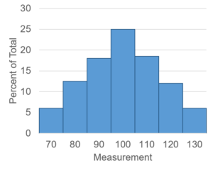
Many times when we measure data and plot it, it looks something like Fig. 5.
Most of the measurements are near the mean, with fewer and fewer measurements as we travel outward in both directions. In statistics we call this mound-shaped data.
Whenever we have mound-shaped data, we can take advantage of a useful application of standard deviation: the Empirical Rule. The Empirical Rule states that in a mound-shaped, symmetric data set, approximately 68{9908f2c9ebc0a4299df98c4fc5aecffecd9da31aa7e644f64ccda5ab2923917a} of the observations fall within 1 standard deviation of the mean, approximately 95{9908f2c9ebc0a4299df98c4fc5aecffecd9da31aa7e644f64ccda5ab2923917a} of the observations fall within 2 standard deviations of the mean, and approximately 99.7{9908f2c9ebc0a4299df98c4fc5aecffecd9da31aa7e644f64ccda5ab2923917a} of the observations fall within 3 standard deviations of the mean (Fig. 6).
An important question to ask about any data set is how much variation there is around the average (mean). This is important for several reasons. For example, two or more samples may have the same mean but have quite different amounts of variation among the observations within each sample. Knowing the variation with a sample, as well as their means and medians, is critical to comparing them statistically. (For more on mean, median, etc., see the Calculating Typical Statistics module.)
Standard Error
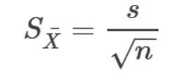
Continuing with our Tetrahymena example, let’s imagine that we have a culture of cells growing for use by our lab. Each person in the lab removes a small sample of the culture, adds black ink, and after 10 minutes, counts the number of food vacuoles formed in each of 20 Tetrahymena. Each person in the lab calculates the mean number of food vacuoles formed. In this scenario, we can say that multiple samples were taken from the same population and measured for the same variable (food vacuole formation). It is quite likely that the means from these samples will not be exactly the same, rather they will vary somewhat from sample to sample. In order to measure the accuracy of the mean, we can use standard error. To calculate standard error, we divide the standard deviation by the square root of the number of samples in our data set. The standard error will always be smaller than the standard deviation.
In our Tetrahymena example above, we calculated a standard deviation of 1.87 for number of food vacuoles counted from 20 different cells. Therefore, the standard error = 1.87/√20 = 1.87/4.47 = 0.418. The formula for the standard error of the mean is shown in Fig. 7.
Often, the terms standard error and standard deviation are confused with each other. It is extremely important to distinguish the two. These two quantities describe very different aspects of our data. The standard deviation describes the dispersion of the data, while the standard error describes the unreliability in the mean of the sample. Another way to think about standard error is that it represents the accuracy, or confidence of the sample; whereas, standard deviation can be thought of as the variation within the sample.
Standardizing Observations
Z-Scores
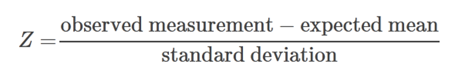
The standard score of an observation (data point) determines the number of standard deviations between the observation (data point) and the mean (average of all data points). This value is also called the z-score (Fig. 8). By converting observed measurements to z-scores, we can say we have standardized the observations.
Why bother standardizing our data? The main advantage of z-scores is that the standardized values are now “on the same scale” and we can directly compare them. Let’s look at an example related to the height of various horse breeds.
Example: Height of Horse Breeds
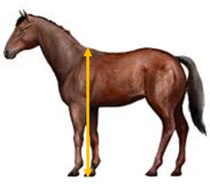
The height of horses is measured in “hands” from the ground to the highest point of their withers (yellow arrow). One hand is 4 inches, or just over 10 cm. Arabian horses range from 14.1 – 15.1 hands, Thoroughbreds 15.2 – 17 hands, and Clydesdales are typically 16 – 18 hands.
Let’s consider some hypothetical (but plausible) data:
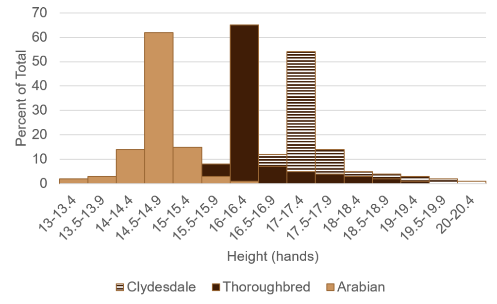
Suppose we have data sets on the height distributions of Arabian, Thoroughbred, and Clydesdale horses (Fig. 10).
From those data, we calculate the following means and standard deviations:
Mean Arabian height = 14.6 hands (58.4 inches) with a standard deviation of 2 inches.
Mean Thoroughbred height = 16.1 hands (64.4 inches) with a standard deviation of 3.6 inches.
Mean Clydesdale height = 17 hands (68 inches) with a standard deviation of 4 inches.
Let’s also suppose that we have an Arabian horse called Gus who is 12 hands tall. How does Gus’ height compare to other Arabian horses?

To answer this question, we can calculate the z-score for Gus’ height. We will need to know Gus’ height, the mean height for Arabian horses, and the standard deviation for Arabian horse height and plug those values into the z-score equation (Fig. 8). We need to make sure that all of our values have the same units. For this example, let’s convert hands to inches.
Z = (observed measurement – expected mean)/standard deviation
Z = (Gus’ height – Arabian horse height mean)/standard deviation of Arabian horse height
Z = (48 inches – 58.4 inches)/2 inches
Z = -10.4/2
Z = -5.2
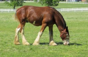
Let’s have a look at another one of our fine horses, Bonnie, a 17.3-hand Clydesdale. How does Bonnie’s height compare to other Clydesdale horses?
Z = (observed measurement – expected mean)/standard deviation
Z = (69.2 inches – 68 inches)/4 inches
Z = 1.2/4
Z = 0.3
How do we interpret our z-score results?
The z-score tells us how many standard deviations our observed measurement is above (for positive z-scores) or below (for negative z-scores). In Gus’ case, his height is 5.2 standard deviations below the mean Arabian horse height. Gus is, in fact, quite small for an Arabian horse (but still fast as lightning). Bonnie, on the other hand, has a z-score of 0.3, meaning she is just a little bit taller than the average Clydesdale.
If we were to directly compare Gus’ height in hands or inches to Bonnie’s height, the comparison would not be very meaningful because each breed has a different distribution of heights and a different average height. By converting each horse’s height to a z-score, we can compare them on an even scale.
References
Chance BL and Rossman AJ (2005). Investigating Statistical Concepts, Applications, and Methods, 1st edition. Duxbury Press. ISBN 0495050644.
Academy K (2012). “Statistics: Standard Deviation.” http://www.khanacademy.org/math/statistics/v/statistics–standard-deviation.
Klug WS, Cummings MR, Spencer CA and Palladino MA (2009). Essentials of Genetics, 7 edition. Benjamin Cummings. ISBN 0321618696.
Molles MC (2007). Ecology – Concepts and Applications (4th, Fourth Edition) By Manuel C. Molles, 4th edition. McGrawHill.
Samuels ML, Witmer JA and Schaffner A (2011). Statistics for the Life Sciences, 4 edition. Addison Wesley. ISBN 0321652800.